<?xml version="1.0" encoding="utf-8"?><feed xmlns="http://www.w3.org/2005/Atom" ><generator uri="https://jekyllrb.com/" version="4.4.1">Jekyll</generator><link href="https://ryan99han.com/feed.xml" rel="self" type="application/atom+xml" /><link href="https://ryan99han.com/" rel="alternate" type="text/html" /><updated>2026-05-30T19:47:22+00:00</updated><id>https://ryan99han.com/feed.xml</id><title type="html">Ryan Han</title><subtitle>Personal website</subtitle><entry><title type="html">Variational Autoencoders</title><link href="https://ryan99han.com/2026/05/23/vae/" rel="alternate" type="text/html" title="Variational Autoencoders" /><published>2026-05-23T00:00:00+00:00</published><updated>2026-05-23T00:00:00+00:00</updated><id>https://ryan99han.com/2026/05/23/vae</id><content type="html" xml:base="https://ryan99han.com/2026/05/23/vae/"><![CDATA[<p><a href="https://arxiv.org/pdf/1312.6114">Auto-Encoding Variational Bayes</a></p>

<p>Solves the problem of training probabilistic models efficiently when the underlying mathematics is intractable, and introduced the variational autoencoder (VAE)</p>

<hr />

<h2 id="background">Background</h2>
<h3 id="latent-variable-z">Latent Variable $z$</h3>
<ul>
  <li>A latent variable $z$ is a hidden factor that explains observed data
    <ul>
      <li>“Hidden” means not explicitly given to the model as an observed variable</li>
    </ul>
  </li>
  <li>For an image dataset, the observed variable is the raw pixels of image $x$</li>
  <li>However, the image may have hidden explanatory factors that determine what we see including lighting, camera angle, zoom level, background, etc.</li>
  <li>The model compresses these hidden factors into the latent variable $z$</li>
  <li>For example with the MNIST image dataset, if $x$ is a handwritten image of a “3”, then the latent variable $z$ might encode things like digit identity, rotation, writing style, etc.</li>
  <li>Latent variables matter because, instead of memorizing pixels, the model learns what underlying causes could have produced the image</li>
</ul>

<h3 id="prior-over-latent-variables-pz">Prior over Latent Variables $p(z)$</h3>
<ul>
  <li>The prior defines what latent vectors are considered likely before seeing the data</li>
  <li>In VAEs, the prior is usually Gaussian: $p(z) = \mathcal{N}(0,1)$
    <ul>
      <li>A Gaussian prior is smooth, continuous, and easy to sample from</li>
      <li>Furthermore, nearby latent points decode into similar outputs</li>
    </ul>
  </li>
</ul>

<h3 id="decoder--generative-model-p_thetax-mid-z">Decoder / Generative Model $p_\theta(x \mid z)$</h3>
<ul>
  <li>This is the neural network that generates data</li>
  <li>$\theta$ represents the parameters (weights and biases) of the model</li>
  <li>$p_{\theta}(x \mid z)$ represents the probability of generating data $x$, given the latent vector $z$, modeled by a network with parameters $\theta$</li>
  <li>This is a generative model because we can generate new data in two steps
    <ul>
      <li>Sample a latent vector $z \sim p(z)$</li>
      <li>Decode the latent vector $x \sim p_{\theta}(x \mid z)$
        <ul>
          <li>The latent vector is inputted into the generative model which outputs a distribution over possible outputs from which $x$ is sampled from</li>
        </ul>
      </li>
    </ul>
  </li>
</ul>

<h3 id="normal-autoencoders">Normal Autoencoders</h3>
<ul>
  <li>Normal autoencoders only learn $x \to z \to x$ by minimizing reconstruction error</li>
  <li>However, this does not guarantee a meaningful latent space</li>
  <li>In a meaningful latent space, nearby latent points correspond to similar data e.g. moving in one direction rotates the face or increases the smile</li>
  <li>For VAEs, you want to sample from a latent space $z \sim p(z)$ and then decode to generate new data</li>
  <li>In a normal autoencoder, random latent variables are usually nonsense because the encoder only used tiny isolated regions of latent space–most of the latent space was never trained on</li>
  <li>A regular autoencoder learns deterministic encoding and decoding but CANNOT answer how likely an image is to be generated by a model</li>
</ul>

<hr />

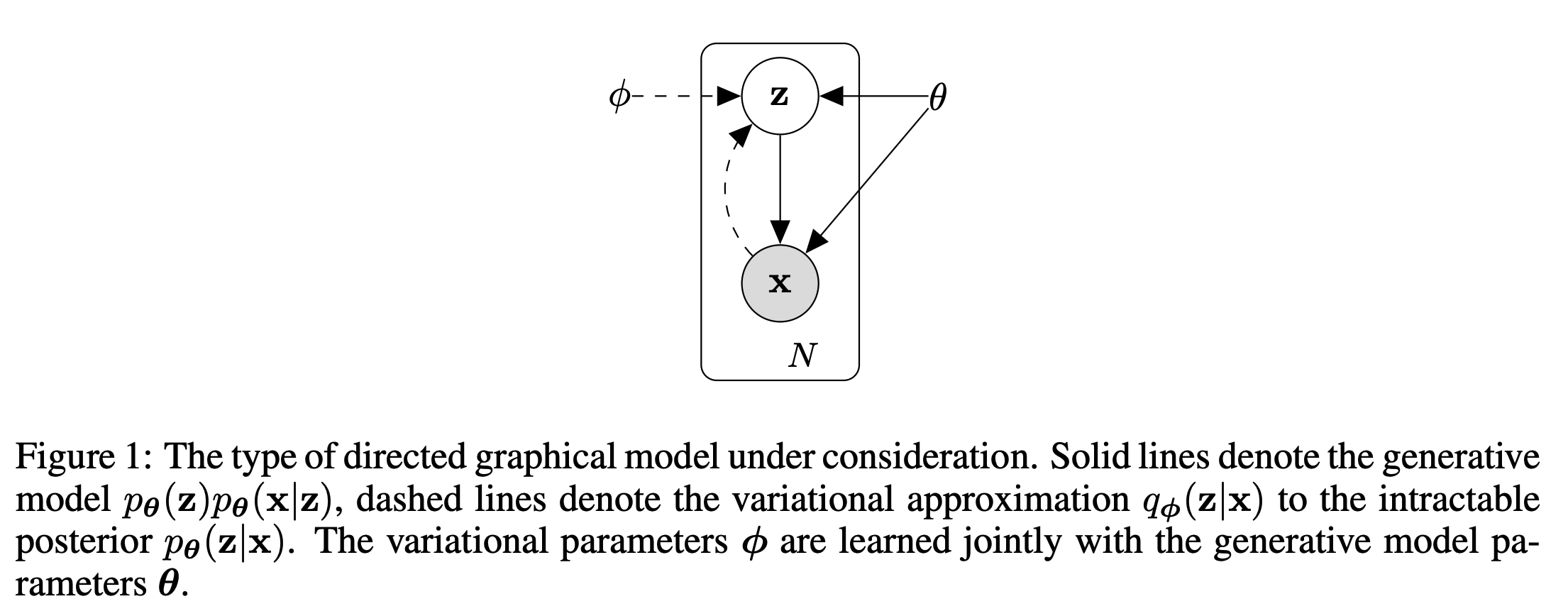
<p><img src="/assets/images/vae.png" alt="VAE" /></p>

<h2 id="mental-model">Mental Model</h2>
<p>A VAE can be considered as:</p>
<ul>
  <li>Encoder: compress input into a Gaussian distribution</li>
  <li>Sample: pick a latent vector from the Gaussian distribution</li>
  <li>Decoder: reconstruct input from the sampled latent vector</li>
  <li>Loss: Balance reconstruction accuracy and latent space regularity</li>
</ul>

<h2 id="intractability">Intractability</h2>
<ul>
  <li>In generative modeling, the observed data $x$ is generated by hidden latent variables $z$</li>
  <li>Given training data, we want to find the parameter $\theta$ that maximizes the probability of our data</li>
  <li>To compute the probability of an observed image $x$, we must consider all possible latent variables that could have produced it</li>
</ul>

<div class="kdmath">$$
p_{\theta}(x) = \int p_{\theta}(x \mid z) p_{\theta}(z) \, dz
$$</div>

<ul>
  <li>However, this integral is impossible to compute because $z$ is high dimensional, $p_\theta$ is a neural network, and there is no algebraic structure to exploit</li>
  <li>We would like to calculate the posterior $p_{\theta}(z \mid x)$ but by Bayes’ rule, $p_{\theta}(z \mid x) = \frac{p_{\theta}(x \mid z)p(z)}{p_\theta(x)}$, and the denominator is intractable</li>
</ul>

<h2 id="variational-inference">Variational Inference</h2>
<ul>
  <li>Since we can’t calculate the true posterior $p_{\theta}(z \mid x)$, we can approximate it with a second distribution $q_{\phi}(z \mid x)$, parameterized by a neural network (the encoder)
    <ul>
      <li>True posterior: $p_{\theta}(z \mid x)$ (unknown, complex)</li>
      <li>Approximate posterior: $q_{\phi}(z \mid x)$ (known, usually Gaussian, predicted by a neural network)</li>
    </ul>
  </li>
</ul>

<h2 id="evidence-lower-bound-elbo">Evidence Lower Bound (ELBO)</h2>
<ul>
  <li>We want to find the parameters $\theta$ which maximize the probability of our data $p_\theta(x)$</li>
</ul>

<div class="kdmath">$$
p_{\theta}(x) = \int p_{\theta}(x \mid z) p_{\theta}(z) \, dz
$$</div>

<div class="kdmath">$$
p_{\theta}(x) = \int p_{\theta}(x, z)dz
$$</div>

<ul>
  <li>Since log is a monotonic function that keeps the optimum the same, but makes the math and optimization much easier we will maximize $\log(p_\theta(x))$</li>
</ul>

<div class="kdmath">$$
\log p_{\theta}(x) = \log \int p_{\theta}(x, z)dz
$$</div>

<ul>
  <li>Multiple and divide by $q_{\phi}(z \mid x)$</li>
</ul>

<div class="kdmath">$$
\log p_{\theta}(x) = \log \int q_{\phi}(z \mid x) \frac{p_{\theta}(x, z)}{q_{\phi}(z \mid x)}dz
$$</div>

<ul>
  <li>We know that for any probaiblity density $q(z)$</li>
</ul>

<div class="kdmath">$$
\mathbb{E}_{q(z \mid x)}[f(z)] = \int q(z)f(z)dz
$$</div>

<ul>
  <li>Then we can rewrite our integral as an expectation</li>
</ul>

<div class="kdmath">$$
\int q_{\phi}(z \mid x) \frac{p_{\theta}(x, z)}{q_{\phi}(z \mid x)}dz = \mathbb{E}_{q_\phi(z \mid x)}\left[\frac{p_{\theta}(x, z)}{q_{\phi}(z \mid x)}\right]
$$</div>

<div class="kdmath">$$
p_{\theta}(x) = \mathbb{E}_{q_\phi(z \mid x)}\left[\frac{p_{\theta}(x, z)}{q_{\phi}(z \mid x)}\right]
$$</div>

<div class="kdmath">$$
\log p_{\theta}(x) = \log \mathbb{E}_{q_\phi(z \mid x)}\left[\frac{p_{\theta}(x, z)}{q_{\phi}(z \mid x)}\right]
$$</div>

<div class="kdmath">$$
f(z) = \frac{p_{\theta}(x, z)}{q_{\phi}(z \mid x)}
$$</div>

<div class="kdmath">$$
\log p_{\theta}(x) = \log \mathbb{E}_{q_\phi(z \mid x)}[f(z)]
$$</div>

<ul>
  <li>Since log is concave, we can use Jensen’s inquality</li>
</ul>

<div class="kdmath">$$
\log \mathbb{E}[f(z)] \geq \mathbb{E}[\log f(z)]
$$</div>

<div class="kdmath">$$
\log \mathbb{E}_{q_\phi(z \mid x)}[f(z)] \geq \mathbb{E}_{q_\phi(z \mid x)}[\log f(z)]
$$</div>

<div class="kdmath">$$
\log p_{\theta}(x) \geq \mathbb{E}_{q_\phi(z \mid x)}[\log f(z)]
$$</div>

<div class="kdmath">$$
\log p_{\theta}(x) \geq \mathbb{E}_{q_\phi(z \mid x)}\left[\log \frac{p_{\theta}(x, z)}{q_{\phi}(z \mid x)}\right]
$$</div>

<ul>
  <li>We call this the evidence lower bound (ELBO)</li>
</ul>

<div class="kdmath">$$
\mathcal{L}_{\theta,\phi;x} = \mathbb{E}_{q_\phi(z \mid x)}\left[\log \frac{p_{\theta}(x, z)}{q_{\phi}(z \mid x)}\right]
$$</div>

<ul>
  <li>While $\log p_\theta(x)$ is intractable, $\mathcal{L}_{\theta,\phi;x}$ is a tractable lower bound we can compute and optimize</li>
</ul>

<h2 id="kl-divergence">KL Divergence</h2>

<ul>
  <li>We have the true posterior $p_{\theta}(z \mid x)$ and the approximate posterior $q_{\phi}(z \mid x)$</li>
  <li>By definition</li>
</ul>

<div class="kdmath">$$
D_{KL}(q_\phi(z \mid x) \| p_\theta(z \mid x)) = \mathbb{E}_{q_\phi(z \mid x)}\left[\log \frac{q_\phi(z \mid x)}{p_\theta(z \mid x)}\right]
$$</div>

<ul>
  <li>
    <p>Since KL divergence is always nonnegative, $KL \geq 0$</p>
  </li>
  <li>
    <p>Baye’s rule says</p>
  </li>
</ul>

<div class="kdmath">$$
p_\theta(z | x) = \frac{p_\theta(x,z)}{p_\theta(x)}
$$</div>

<ul>
  <li>Then</li>
</ul>

<div class="kdmath">$$
KL = \mathbb{E}_{q_\phi(z \mid x)}\left[\log \frac{q_\phi(z \mid x)p_\theta(x)}{p_\theta(x,z)}\right]
$$</div>

<div class="kdmath">$$
KL = \mathbb{E}_{q_\phi(z \mid x)} [\log q_\phi(z \mid x) + \log p_\theta(x) - \log p_\theta(x,z)]
$$</div>

<ul>
  <li>Since $\log p_\theta(x)$ does not depend on $z$</li>
</ul>

<div class="kdmath">$$
\mathbb{E}_{q_\phi(z \mid x)} [\log p_\theta(x)] = \log p_\theta(x)
$$</div>

<div class="kdmath">$$
KL = \log p_\theta(x) + \mathbb{E}_{q_\phi(z \mid x)} [\log q_\phi(z \mid x)] - \mathbb{E}_{q_\phi(z \mid x)}[\log p_\theta(x,z)]
$$</div>

<ul>
  <li>Rearranging</li>
</ul>

<div class="kdmath">$$
\log p_\theta(x) = \mathbb{E}_{q_\phi(z \mid x)}[\log p_\theta(x,z)] - \mathbb{E}_{q_\phi(z \mid x)} [\log q_\phi(z \mid x)] + KL
$$</div>

<div class="kdmath">$$
\log p_\theta(x) = \mathbb{E}_{q_\phi(z \mid x)}\left[\frac{\log p_\theta(x,z)}{\log q_\phi(z \mid x)}\right] + KL
$$</div>

<div class="kdmath">$$
\log p_\theta(x) = \mathbb{E}_{q_\phi(z \mid x)}\left[\frac{\log p_\theta(x,z)}{\log q_\phi(z \mid x)}\right] + D_{KL}(q_\phi(z \mid x) \| p_\theta(z \mid x))
$$</div>

<ul>
  <li>The first term is exactly the ELBO!</li>
</ul>

<div class="kdmath">$$
\mathcal{L}(x; \theta, \phi) = \mathbb{E}_{q_\phi(z \mid x)}\left[\frac{\log p_\theta(x,z)}{\log q_\phi(z \mid x)}\right]
$$</div>

<div class="kdmath">$$
\log p_\theta(x) = \mathcal{L}(x; \theta, \phi) + D_{KL}(q_\phi(z \mid x) \| p_\theta(z \mid x))
$$</div>

<ul>
  <li>Because the KL divergence is always nonnegative, the ELBO is automatically a lower bound</li>
</ul>

<div class="kdmath">$$
\mathcal{L}(x; \theta, \phi) \leq \log p_\theta(x)
$$</div>

<ul>
  <li>And the gap between the ELBO and the true log-likelihood is exactly the error in the posterior!</li>
</ul>

<div class="kdmath">$$
D_{KL}(q_\phi(z \mid x) \| p_\theta(z \mid x)) = 0 \to \log p_\theta(x) = \mathcal{L}(x; \theta, \phi)
$$</div>

<ul>
  <li>So maximizing the ELBO data likelihood does two things simultaneously:
    <ul>
      <li>1) Increases data likelihood</li>
      <li>2) Makes encoder approximate the true posterior</li>
    </ul>
  </li>
</ul>

<h2 id="vae-loss">VAE Loss</h2>

<div class="kdmath">$$
\log p_\theta(x) = \mathcal{L}(x; \theta, \phi) + D_{KL}(q_\phi(z \mid x) \| p_\theta(z \mid x))
$$</div>

<ul>
  <li>This form is still unusable since</li>
</ul>

<div class="kdmath">$$
p_\theta(z \mid x) = \frac{p_\theta(x \mid z)p(z)}{p_\theta(x)}
$$</div>

<div class="kdmath">$$
p_\theta(x) = \int p_{\theta}(x \mid z)p(z)dz
$$</div>

<ul>
  <li>So we’ll expand the KL term</li>
</ul>

<div class="kdmath">$$
D_{KL}(q_\phi(z \mid x) \| p_\theta(z \mid x)) = \mathbb{E}_{q_\phi} \left[\log \frac{q_\phi(z \mid x)}{p_\theta(z \mid x)} \right]
$$</div>

<div class="kdmath">$$
KL = \mathbb{E}_{q_\phi} \left[\log \frac{q_\phi(z \mid x)}{p_\theta(z \mid x)} \right]
$$</div>

<ul>
  <li>From Baye’s rule</li>
</ul>

<div class="kdmath">$$
p_\theta(z \mid x) = \frac{p_\theta(x,z)}{p_\theta(x)}
$$</div>

<ul>
  <li>Substitute back into the KL equation</li>
</ul>

<div class="kdmath">$$
KL = \mathbb{E}_{q_\phi} \left[\log \frac{q_\phi(z \mid x)p_\theta(x)}{p_\theta(x,z)} \right]
$$</div>

<div class="kdmath">$$
KL = \mathbb{E}_{q_\phi} [\log q_\phi(z \mid x) + \log p_\theta(x) - \log p_\theta(x,z)]
$$</div>

<div class="kdmath">$$
KL = \mathbb{E}_{q_\phi} [\log q_\phi(z \mid x)] - \mathbb{E}_{q_\phi} [\log p_\theta(x,z)] + \log p_\theta(x)
$$</div>

<ul>
  <li>Recall from earlier</li>
</ul>

<div class="kdmath">$$
\log p_\theta(x) = ELBO + KL
$$</div>

<div class="kdmath">$$
\log p_\theta(x) = ELBO + \mathbb{E}_{q_\phi} [\log q_\phi(z \mid x)] - \mathbb{E}_{q_\phi} [\log p_\theta(x,z)] + \log p_\theta(x)
$$</div>

<ul>
  <li>Rearrange for ELBO</li>
</ul>

<div class="kdmath">$$
ELBO = \mathbb{E}_{q_\phi} [\log p_\theta(x,z)] - \mathbb{E}_{q_\phi} [\log q_\phi(z \mid x)]
$$</div>

<div class="kdmath">$$
p_\theta(x,z) = p_\theta(x \mid z)p_\theta(z)
$$</div>

<div class="kdmath">$$
ELBO = \mathbb{E}_{q_\phi} [\log p_\theta(x \mid z)p_\theta(z)] - \mathbb{E}_{q_\phi} [\log q_\phi(z \mid x)]
$$</div>

<div class="kdmath">$$
ELBO = \mathbb{E}_{q_\phi} [\log p_\theta(x \mid z)] + \mathbb{E}_{q_\phi} [\log p_\theta(z)] - \mathbb{E}_{q_\phi} [\log q_\phi(z \mid x)]
$$</div>

<div class="kdmath">$$
ELBO = \mathbb{E}_{q_\phi} [\log p_\theta(x \mid z)] + \mathbb{E}_{q_\phi} \left[\log \frac{p_\theta(z)}{q_\phi(z \mid x)}\right]
$$</div>

<ul>
  <li>From the definition of KL divergence</li>
</ul>

<div class="kdmath">$$
\mathbb{E}_{q_\phi} \left[\log \frac{p_\theta(z)}{q_\phi(z \mid x)}\right] = -KL(q_\phi(z \mid x)||p(z))
$$</div>

<div class="kdmath">$$
ELBO = \mathbb{E}_{q_\phi(z \mid x)} [\log p_\theta(x \mid z)] - KL(q_\phi(z \mid x)||p(z))
$$</div>

<h2 id="reparameterization-trick">Reparameterization Trick</h2>
<ul>
  <li>The encoder’s job is to output two numbers: a mean $\mu$ and standard deviation $\sigma$, in essence spitting out a cloud of probability in which the image lives</li>
  <li>We sample a point $z$ from that probability cloud</li>
  <li>The decoder takes $z$ and tries to rebuild the image</li>
  <li>To steer the reconstruction in the right direction, gradients need to be propagated backwards</li>
  <li>However, the encoder didn’t output $z$ directly, only $\mu$ and $\sigma$</li>
  <li>If we treat sampling as a black box operation of sampling $z$ from $\mathcal{N}(\mu, \sigma^2)$, there is no mathematical link between $z$ and $\mu$, breaking the chain rule</li>
  <li>Instead of sampling $z$ directly from $\mathcal{N}(\mu, \sigma^2)$, we express $z$ as a deterministic transformation of noise $\epsilon$:</li>
</ul>

<div class="kdmath">$$
z = \mu + \sigma \odot \epsilon, \quad \epsilon \sim \mathcal{N}(0, I)
$$</div>

<ul>
  <li>Now $z$ is a function of parameters $(\mu, \sigma)$ and fixed noise $\epsilon$, so we can take gradients with respect to $\mu$ and $\sigma$ while treating $\epsilon$ as a constant</li>
</ul>

<h2 id="architecture">Architecture</h2>
<ul>
  <li><strong>Input:</strong> Data point $x$</li>
  <li><strong>Encoder (Recognition Model):</strong> Neural network outputs parameters $\mu$ and $\log(\sigma^2)$</li>
  <li><strong>Latent Space:</strong> Apply reparameterization trick $z = \mu + \sigma \odot \epsilon$</li>
  <li><strong>Decoder (Generative Model):</strong> Neural network takes $z$ and outputs parameters to reconstruct $x$ (e.g. pixels)</li>
  <li><strong>Loss:</strong> Calculate ELBO and backpropagate to update weights in both encoder and decoder</li>
</ul>]]></content><author><name></name></author><category term="Papers" /><summary type="html"><![CDATA[Auto-Encoding Variational Bayes]]></summary></entry><entry><title type="html">Residual Networks</title><link href="https://ryan99han.com/2026/05/20/resnet/" rel="alternate" type="text/html" title="Residual Networks" /><published>2026-05-20T00:00:00+00:00</published><updated>2026-05-20T00:00:00+00:00</updated><id>https://ryan99han.com/2026/05/20/resnet</id><content type="html" xml:base="https://ryan99han.com/2026/05/20/resnet/"><![CDATA[<p><a href="https://arxiv.org/pdf/1512.03385">Deep Residual Learning for Image Recognition</a></p>

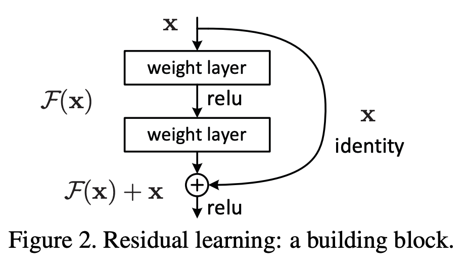
<p>Learning residual functions significantly improves quality when training deep neural networks</p>

<p><img src="/assets/images/resnet.png" alt="ResNet" /></p>

<h2 id="overview">Overview</h2>
<ul>
  <li>Deep convolutional neural networks have led to major breakthroughs in image classification, in large part due to increasing the depth of the network</li>
  <li>However, there are two issues when simply stacking more layers
    <ul>
      <li>Vanishing gradients</li>
      <li>Degradation</li>
    </ul>
  </li>
  <li>Vanishing Gradients
    <ul>
      <li>Vanishing gradients refer to when the gradients of earlier layers become very close to zero, leading to updates of the weights also becoming very close to zero</li>
      <li>This leads to:
        <ul>
          <li>Stagnant learning in the earlier layers, which are crucial for learning fundamental features (edges, patterns, etc.)</li>
          <li>Poor feature extraction and learning in the deeper layers since they build upon features learned in the early layers</li>
        </ul>
      </li>
      <li>
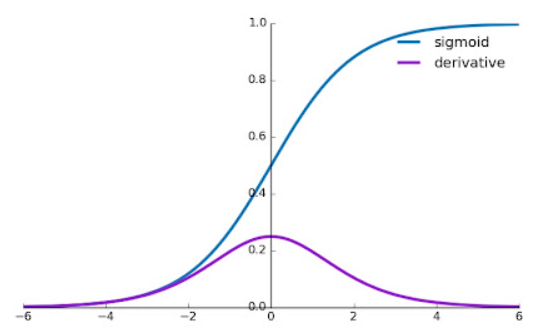
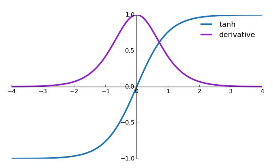
        <p>The vanishing gradient problem often arises when using certain activation functions like the sigmoid function or hyperbolic tangent (tanh) function</p>

        <p><img src="/assets/images/sigmoid.png" alt="Sigmoid" style="width:40%; display:inline-block; margin-right:2%" /> <img src="/assets/images/tanh.png" alt="Tanh" style="width:40%; display:inline-block" /></p>
      </li>
      <li>For large positive or negative inputs to the sigmoid function, the sigmoid function “saturates” near 0 or 1, where the derivative is a very small positive number</li>
      <li>For large positive or negative inputs to the tanh function, the tanh function “saturates” near -1 or 1, where the derivative is a very small positive number.</li>
      <li>During backpropagation, the local gradients are continually multiplied together, shrinking the values towards zero</li>
      <li>Vanishing gradients are largely solved by techniques like:
        <ul>
          <li>Rectified Linear Unit (ReLU) activation function whose derivative is 1 for all positive inputs
            <ul>
              <li>$ReLU(x) = max(0, x)$</li>
            </ul>
          </li>
          <li>Normalized initialization and intermediate normalization layers</li>
          <li>Residual networks (this paper)</li>
        </ul>
      </li>
    </ul>
  </li>
  <li>Degradation
    <ul>
      <li>As the depth of the network increases, accuracy saturates and then degrades rapidly</li>
      <li>Unexpectedly, this is <strong>not</strong> caused by overfitting, and adding more layers leads to higher training error</li>
    </ul>
  </li>
</ul>

<h2 id="residual-networks">Residual Networks</h2>
<ul>
  <li>Instead of hoping a few stacked layers directly fit a desired underlying mapping, we let these layers fit a residual mapping
    <ul>
      <li>Formally, let the underlying desired mapping be $\mathcal{H}(x)$</li>
      <li>Then the stacked nonlinear layers fit a mapping of $\mathcal{F}(x) \coloneqq \mathcal{H}(x) - x$</li>
      <li>The original mapping is now recast into $\mathcal{F}(x) + x$</li>
    </ul>
  </li>
  <li>The hypothesis is that it is easier to optimize the residual mapping than to optimize the original, unreferenced mapping</li>
  <li>To the extreme, if an identity mapping were optimal, it would be easier to push the residual to zero than to fit an identity mapping by a stack of nonlinear layers</li>
  <li>For the implementation, we use shortcut connections which simply perform an identity mapping, and their outputs are added to the outputs of the stacked layers</li>
  <li>Identity shortcut connections add neither extra parameter nor computation complexity</li>
</ul>]]></content><author><name></name></author><category term="Papers" /><summary type="html"><![CDATA[Deep Residual Learning for Image Recognition]]></summary></entry><entry><title type="html">U-Net</title><link href="https://ryan99han.com/2026/05/19/unet/" rel="alternate" type="text/html" title="U-Net" /><published>2026-05-19T00:00:00+00:00</published><updated>2026-05-19T00:00:00+00:00</updated><id>https://ryan99han.com/2026/05/19/unet</id><content type="html" xml:base="https://ryan99han.com/2026/05/19/unet/"><![CDATA[<p><a href="https://arxiv.org/pdf/1505.04597">U-Net: Convolutional Networks for Biomedical Image Segmentation</a></p>

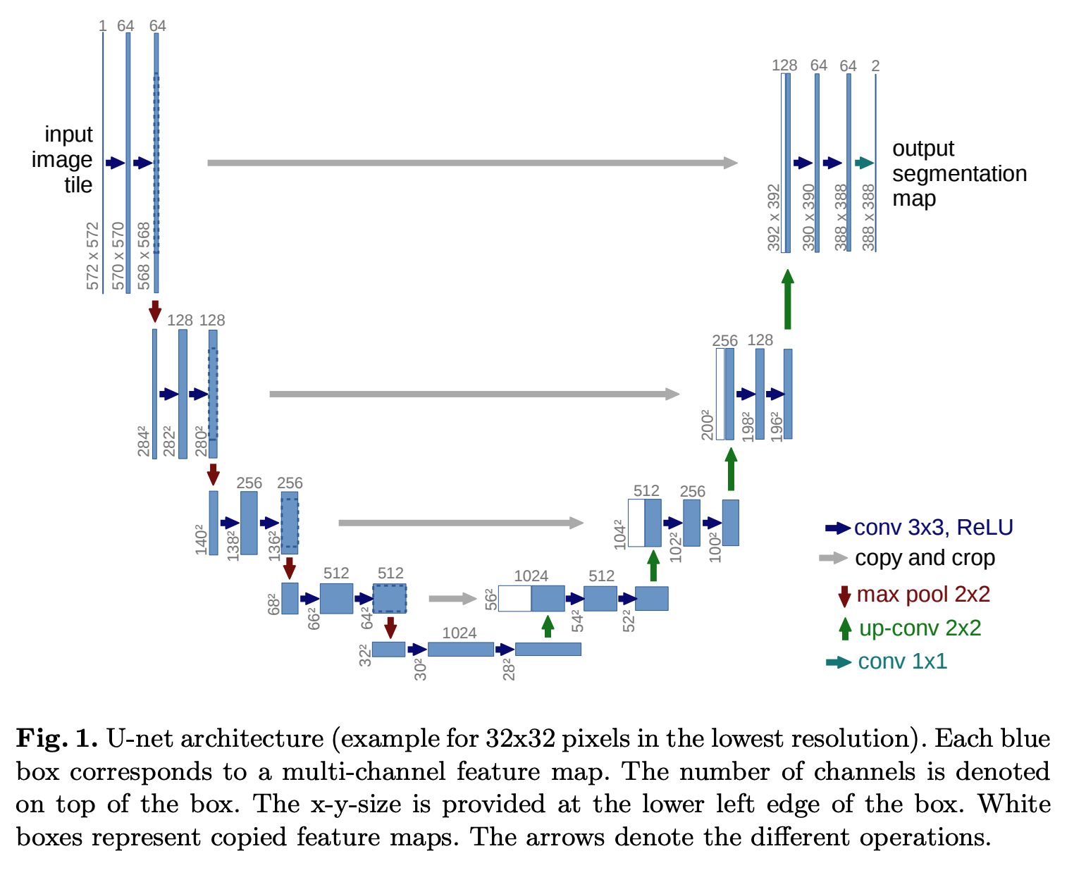
<p>The U-Net is an architecture for convolutional neural networks consisting of an encoder and decoder with skip connections</p>

<p><img src="/assets/images/unet.png" alt="U-Net" /></p>

<h2 id="overview">Overview</h2>
<ul>
  <li>Previous architectures of convolutional networks failed to preserve high-resolution details</li>
  <li>In a standard encoder-decoder network, data is compressed into a bottleneck where spatial information is lost in favor of high-level semantic meaning</li>
  <li>The breakthrough with this paper was the introduction of skip connections, which skip the bottleneck by concatenating feature maps from the encoding path directly to the feature maps in the decoding path
    <ul>
      <li>Preserves high-resolution information of the input image from the encoding path, so the model no longer has to guess about high-resolution details in the decoding path</li>
      <li>Enables fusion of features so the model can leverage both high-level and low-level information</li>
      <li>Improves gradient flow by propagating gradients from output layer back to earlier layers</li>
    </ul>
  </li>
</ul>

<h2 id="encoder">Encoder</h2>
<ul>
  <li>Repeated application of:
    <ul>
      <li>Two $3 \times 3$ convolutions, each followed by ReLU</li>
      <li>$2 \times 2$ max pooling operation with stride 2 for downsampling</li>
      <li>Double the number of feature maps at each downsampling stack</li>
    </ul>
  </li>
</ul>

<h2 id="decoder">Decoder</h2>
<ul>
  <li>Repeated application of:
    <ul>
      <li>
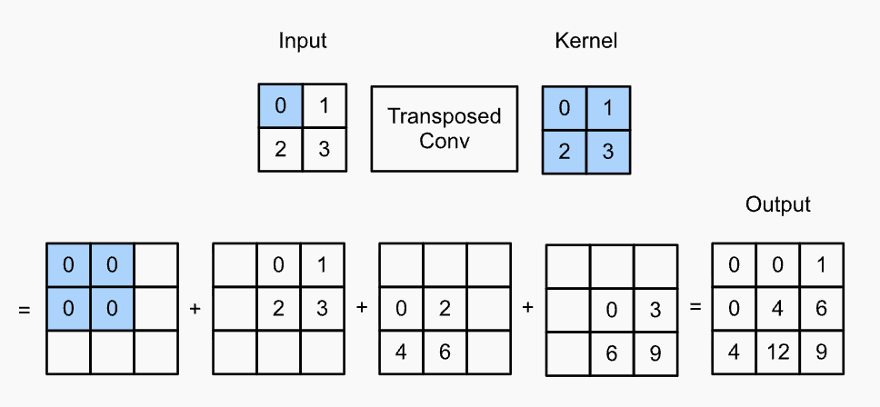
        <p>$2 \times 2$ transposed convolution with stride 2 for upsampling</p>

        <p><img src="/assets/images/transposed_convolution.png" alt="Transposed Convolution" /></p>
      </li>
      <li>Concatenation with cropped feature maps from contracting path</li>
      <li>Channel reduction via 3D filters of dimensions $W \times D \times C$ (width, depth, channels)
        <ul>
          <li>Act as weighted combinations of features from multiple channels</li>
        </ul>
      </li>
      <li>Two $3 \times 3$ convolutions, each followed by ReLU</li>
    </ul>
  </li>
</ul>

<h2 id="breakdown">Breakdown</h2>
<ul>
  <li>Concretely in the encoding path of the image above:
    <ul>
      <li>Start with a grayscale image $572 \times 572 \times 1$</li>
      <li>Apply 64 filters of dimensions $3 \times 3 \times 1$ (&amp; ReLU) $\to 570 \times 570 \times 64$</li>
      <li>Apply 64 filters of dimensions $3 \times 3 \times 64$ (&amp; ReLU) $\to 568 \times 568 \times 64$</li>
      <li>Apply $2 \times 2$ max pooling with stride 2 $\to 284 \times 284 \times 64$</li>
      <li>Apply 128 filters of dimensions $3 \times 3 \times 64$ (&amp; ReLU) $\to 282 \times 282 \times 128$</li>
    </ul>
  </li>
  <li>Concretely in the decoding path of the image above:
    <ul>
      <li>Start at the bottleneck with a feature map of dimensions $28 \times 28 \times 1024$</li>
      <li>Apply 512 transposed filters of dimensions $2 \times 2 \times 1024 \to 56 \times 56 \times 512$</li>
      <li>Concatenate a cropped feature map of $56 \times 56 \times 512 \to 56 \times 56 \times 1024$</li>
      <li>Apply 512 filters of dimensions $3 \times 3 \times 1024$ (&amp; ReLU) $\to 54 \times 54 \times 512$</li>
      <li>Apply 512 filters of dimensions $3 \times 3 \times 512$ (&amp; ReLU) $\to 52 \times 52 \times 512$</li>
      <li>Apply 256 transposed filters of dimensions $2 \times 2 \times 512 \to 104 \times 104 \times 256$</li>
    </ul>
  </li>
</ul>

<h2 id="summary">Summary</h2>
<ul>
  <li>Encoding path:
    <ul>
      <li>Spatial dimensions decrease $\to$ loses precise locations &amp; gains global context</li>
      <li>Channel dimensions increase $\to$ gains complex concept detection</li>
    </ul>
  </li>
  <li>Decoding path:
    <ul>
      <li>Spatial dimensions increase $\to$ recovers spatial resolution</li>
      <li>Channel dimensions decrease $\to$ compresses abstract concepts back into pixels</li>
    </ul>
  </li>
</ul>]]></content><author><name></name></author><category term="Papers" /><summary type="html"><![CDATA[U-Net: Convolutional Networks for Biomedical Image Segmentation]]></summary></entry><entry><title type="html">Convolutional Neural Networks</title><link href="https://ryan99han.com/2026/05/17/cnn/" rel="alternate" type="text/html" title="Convolutional Neural Networks" /><published>2026-05-17T00:00:00+00:00</published><updated>2026-05-17T00:00:00+00:00</updated><id>https://ryan99han.com/2026/05/17/cnn</id><content type="html" xml:base="https://ryan99han.com/2026/05/17/cnn/"><![CDATA[<p><a href="https://arxiv.org/pdf/1511.08458">An Introduction to Convolutional Neural Networks</a></p>

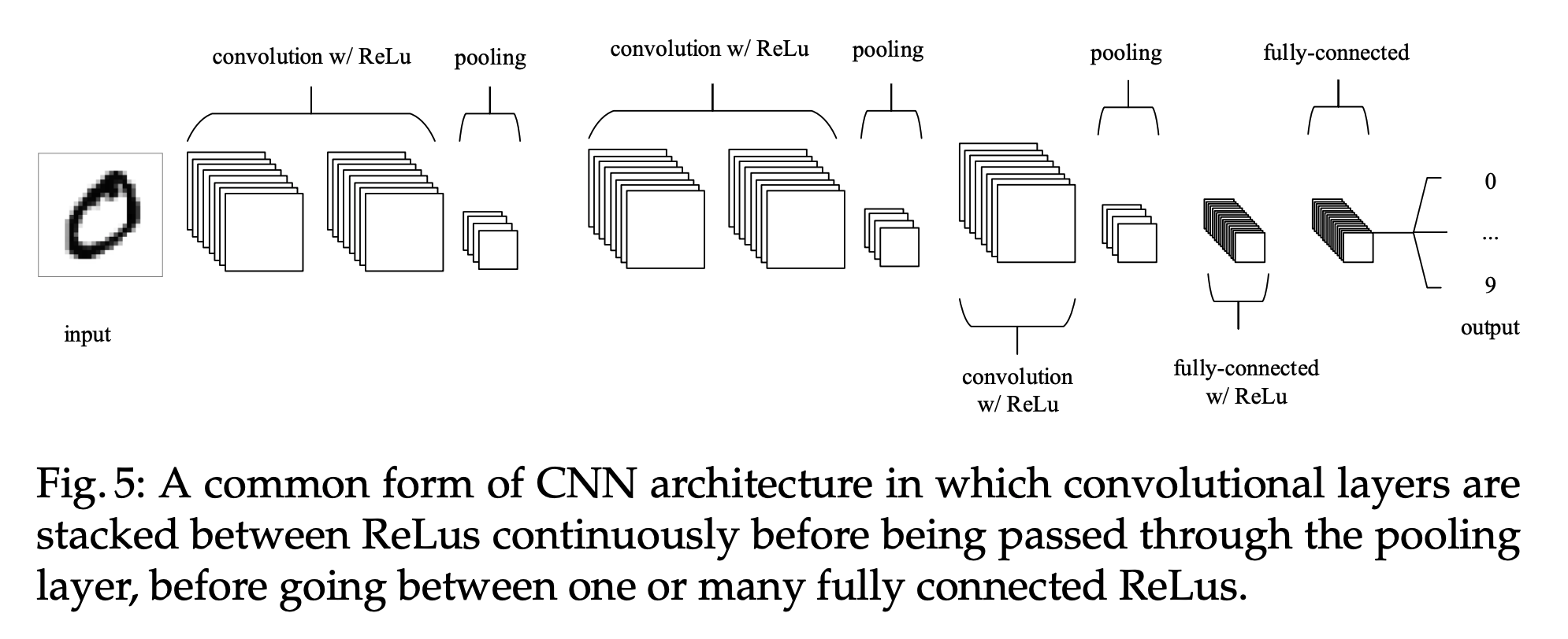
<p>Convolutional neural networks (CNNs) are a type of neural network which use filters glided across the input to detect patterns in images, video, audio, etc.</p>

<p><img src="/assets/images/cnn.png" alt="CNN" /></p>

<h2 id="advantages">Advantages</h2>
<ul>
  <li>Reduces the number of input nodes (less computation and training time)</li>
  <li>Tolerates small shifts of an image (less overfitting)</li>
  <li>Takes advantage of local spatial correlations in images</li>
</ul>

<h2 id="layers">Layers</h2>
<ul>
  <li><strong>Convolutional layers</strong>: convolve a kernel with the input image</li>
  <li><strong>Pooling layers</strong>: downsample the spatial dimensionality</li>
  <li><strong>Fully-connected layers</strong>: traditional neural network architecture</li>
</ul>

<h2 id="convolutional-layer">Convolutional Layer</h2>
<ul>
  <li>Extracts features from an input image using filters (or kernels):
    <ul>
      <li>Small in spatial dimensionality and are overlaid on top of the image with dimensions $(F * F * D_i)$
        <ul>
          <li>$D_i = 3$ for RGB channels</li>
          <li>$D_i = N$ for the number of filters from the previous layer</li>
        </ul>
      </li>
      <li>Glided through the input, where the output is the dot product of the input and filter with the addition of a bias term</li>
      <li>Feature maps are then typically fed through a ReLU function: $f(x) = \max(x,0)$</li>
    </ul>
  </li>
  <li>The weights and bias of the kernel are adjusted via backpropagation during training</li>
  <li>Each cell in a feature map therefore corresponds to a group of neighboring pixels and the network will learn kernels that fire when they see a specific feature at a given spatial position</li>
  <li>Convolutional layers can significantly reduce the complexity of a model through optimizing three hyperparameters:
    <ul>
      <li><strong>Depth</strong>: Number of different kernels convolved across the input volume</li>
      <li><strong>Stride</strong>: How many pixels the filter shifts over the input volume at each step of the convolution</li>
      <li><strong>Padding</strong>: Extra rows and columns of zeros added to the border of the input image or feature map
        <ul>
          <li>Prevents the feature map from shrinking too rapidly (for deeper networks)</li>
          <li>Preserves information from pixels on the edge</li>
        </ul>
      </li>
    </ul>
  </li>
</ul>

<h2 id="pooling-layer">Pooling Layer</h2>
<ul>
  <li>Reduces the dimensionality of the representation by computing some aggregated value over each feature map
    <ul>
      <li>In max pooling, take the largest value in the feature map over the covered area</li>
    </ul>
  </li>
  <li>The outputs of pooling layers are typically the input of a traditional neural network by flattening the 2D feature maps into a single vector of values and concatenating multiple feature maps</li>
</ul>]]></content><author><name></name></author><category term="Papers" /><summary type="html"><![CDATA[An Introduction to Convolutional Neural Networks]]></summary></entry></feed>