Neural Discrete Representation Learning
Proposes a generative model which is based on the variational autoencoder (VAE) but learns discrete representations, instead of continuous ones.
Introduction
- VQ-VAEs differ from VAEs in two ways:
- The encoder outputs discrete, rather than continuous, representations
- The prior is learned not static
- VQ-VAEs have two advantages over VAEs:
- VAEs can suffer from “posterior collapse” in which a powerful decoder completely ignores the latents
- Discrete representations are potentially a better fit for modalities like language or even images (patches)
VAEs
- VAEs consist of:
- Encoder network which parameterises a posterior distribution $q(z \mid x)$ of discrete latent random variables $z$ given the input data $x$
- Prior distribution $p(z)$
- Decoder with distribution $p(x \mid z)$ over input data
Discrete Latent Variables
- Latent embedding space $\epsilon \in R^{KxD}$ where $K$ is the size of the discrete latent space and $D$ is the dimensionality of each latent embedding vector $e_i$
- Thus, there are $K$ embedding vectors $e_i \in R^D$ where $i \in 1, 2, … K$
- The model takes as input $x$ and outputs from the encoder $z_e(x)$
- Nearest-neighbor lookup is used to find the closest embedding vector $e_k$
- Formally, the posterior categorial distribution $q(z \mid x)$ probabilities are defined as:
$$
q(z = k \mid x) = \begin{cases} 1 & \text{for } k = \operatorname{argmin}_j \lVert z_e(x) - e_j \rVert_2, \\ 0 & \text{otherwise} \end{cases}
$$
- Breakdown:
- The encoder output is $z_e(x)$ is the encoder output
- Calculate the Euclidean distance between each of the embedding vectors $e_j$ and $z_e(x)$
- Get the index $k$ of the closest embedding vector $e_k$
- The probability $q(z = k \mid x)$ is 1 for the single index $k$ and 0 for all other indices
- After this mapping,
$$
z_q(x) = e_k \text{ where } k = \operatorname{argmin}_j \lVert z_e(x) - e_j \rVert_2
$$
Learning
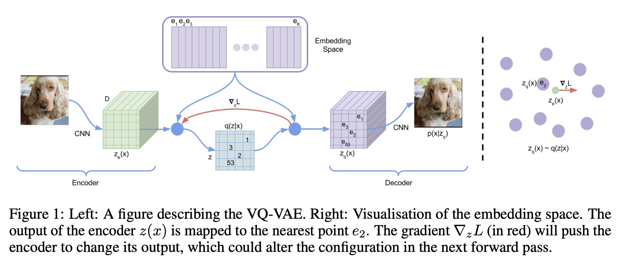
- For backpropagation, nearest-neighbor lookup is not differentiable so the gradients are propagated directly through from the decoder input $z_q(x)$ to encoder output $z_e(x)$ (straight-through estimator)
- The output representation of the encoder and the input to the decoder share the same $D$ dimensional space, so the gradients contain useful information for how the encoder should change its output to lower the reconstruction loss
Loss Function
- Stop-gradient $sg[x]$ is an operation which allows the variable $x$ to be propagated in the forward process, but pretends that $x$ is a constant during backpropagation (no gradient descent on $x$)
- The loss is composed of three parts:
- 1) Reconstruction loss
- Exactly like a normal autoencoder, and can be mean-squared error for images or cross-entropy loss for discrete data
$$
L_{reconstruction} = \log(p \mid z_q(x))
$$
- 2) Codebook loss
- The codebook embeddings should move towards the encoder outputs, improving the dictionary
$$
L_{codebook} = \lVert sg[z_e(x)] - e \rVert ^ 2
$$
- 3) Commitment loss
- Encourage encoder outputs to stay near the selected embedding to stabilize training
- Without this, the encoder could keep changing arbitrarily while the codebook chases it
$$
L_{commitment} = \beta \lVert z_e(x) - sg[e] \rVert ^ 2
$$
- Thus the final loss is:
$$
L = \log p(x \mid z_q(x)) + \lVert sg[z_e(x)] - e \rVert ^ 2 + \beta \lVert z_e(x) - sg[e] \rVert ^ 2
$$
Prior
- First the VQ-VAE is trained, which results in a model that can reconstruct images, but not generate new ones
- This is because the encoder learned to turn an image into a grid of integer (codebook indices), while the decoder learned to turn those grid of integers into an image
- To generate new images, we train a prior by learning sequences of integer codes which make sense
- In the paper, the authors train a PixelCNN to predict these tokens
- This PixelCNN becomes $p(z)$, the prior over latent variables
- Note that a standard VAE assumes that the latent variable $z$ comes from a standard Gaussian distribution and during training, the KL divergence forces every encoded example (image $\to$ latent) to look like samples from the Gaussian
- The latent space is therefore constrained to match a distribution that may not reflect the true structure of the data
- However for VQ-VAEs, the encoder outputs discrete codebook indices, and there is no probability distribution over these indices
- After training, a prior can be learned by pumping many examples through the encoder and training a model to predict the sequences of tokens
- A learned prior can model the actual distribution of latent representations instead of forcing the distribution into a simple Gaussian