Auto-Encoding Variational Bayes
Solves the problem of training probabilistic models efficiently when the underlying mathematics is intractable, and introduces the variational autoencoder (VAE)
Background
Latent Variable $z$
- A latent variable $z$ is a hidden factor that explains observed data
- “Hidden” means not explicitly given to the model as an observed variable
- For an image dataset, the observed variable is the raw pixels of image $x$
- However, the image may have hidden explanatory factors that determine what we see including lighting, camera angle, zoom level, background, etc.
- The model compresses these hidden factors into the latent variable $z$
- For example with the MNIST image dataset, if $x$ is a handwritten image of a “3”, then the latent variable $z$ might encode things like digit identity, rotation, writing style, etc.
- Latent variables matter because, instead of memorizing pixels, the model learns what underlying causes could have produced the image
Prior over Latent Variables $p(z)$
- The prior defines what latent vectors are considered likely before seeing the data
- In VAEs, the prior is usually Gaussian: $p(z) = \mathcal{N}(0,1)$
- A Gaussian prior is smooth, continuous, and easy to sample from
- Furthermore, nearby latent points decode into similar outputs
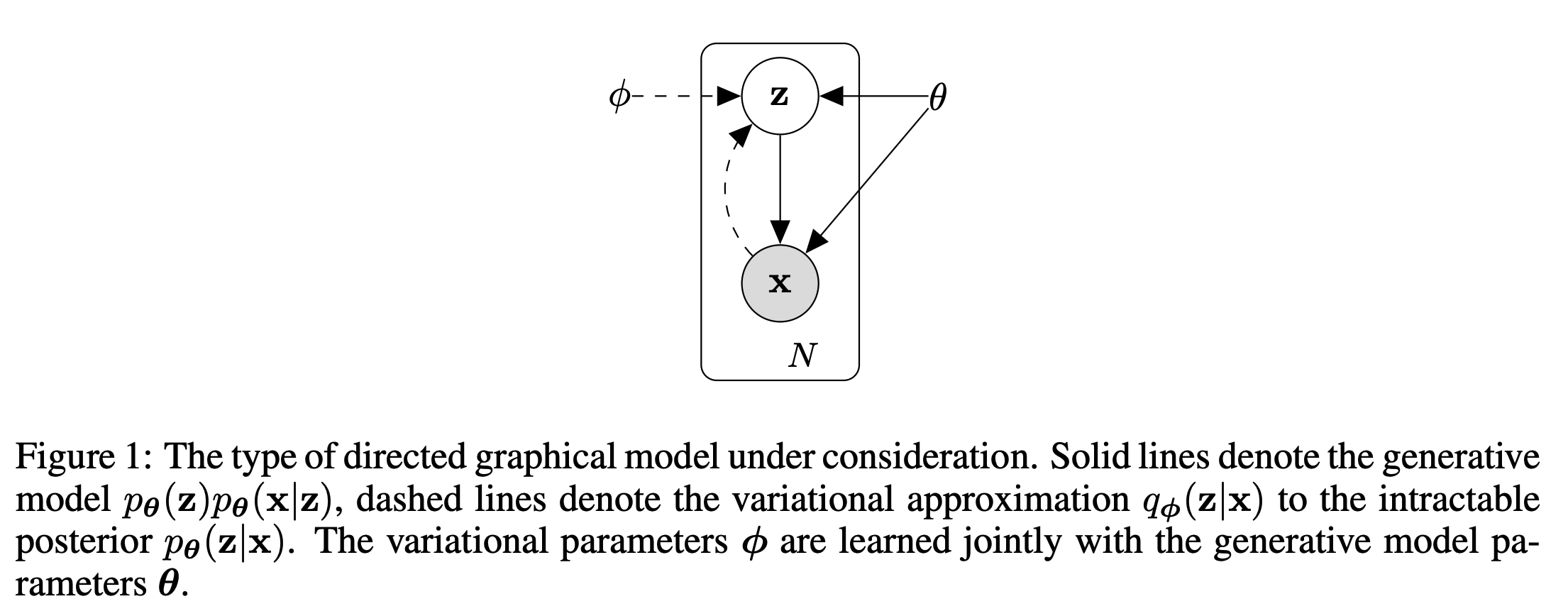
Decoder / Generative Model $p_\theta(x \mid z)$
- This is the neural network that generates data
- $\theta$ represents the parameters (weights and biases) of the model
- $p_{\theta}(x \mid z)$ represents the probability of generating data $x$, given the latent vector $z$, modeled by a network with parameters $\theta$
- This is a generative model because we can generate new data in two steps
- Sample a latent vector $z \sim p(z)$
- Decode the latent vector $x \sim p_{\theta}(x \mid z)$
- The latent vector is inputted into the generative model which outputs a distribution over possible outputs from which $x$ is sampled from
Normal Autoencoders
- Normal autoencoders only learn $x \to z \to x$ by minimizing reconstruction error
- However, this does not guarantee a meaningful latent space
- In a meaningful latent space, nearby latent points correspond to similar data e.g. moving in one direction rotates the face or increases the smile
- For VAEs, you want to sample from a latent space $z \sim p(z)$ and then decode to generate new data
- In a normal autoencoder, random latent variables are usually nonsense because the encoder only uses tiny isolated regions of latent space–most of the latent space was never trained on
- A regular autoencoder learns deterministic encoding and decoding but CANNOT answer how likely an image is to be generated by a model
Mental Model
A VAE can be considered as:
- Encoder: compress input into a Gaussian distribution
- Sample: pick a latent vector from the Gaussian distribution
- Decoder: reconstruct input from the sampled latent vector
- Loss: Balance reconstruction accuracy and latent space regularity
Intractability
- In generative modeling, the observed data $x$ is generated by hidden latent variables $z$
- Given training data, we want to find the parameter $\theta$ that maximizes the probability of our data
- To compute the probability of an observed image $x$, we must consider all possible latent variables that could have produced it
$$
p_{\theta}(x) = \int p_{\theta}(x \mid z) p_{\theta}(z) \, dz
$$
- However, this integral is impossible to compute because $z$ is high dimensional, $p_\theta$ is a neural network, and there is no algebraic structure to exploit
- We would like to calculate the posterior $p_{\theta}(z \mid x)$ because doing so would allow us to map real-world data into a compact and meaningful latent space where we can reason about its underlying properties
- However, by Bayes’ rule, $p_{\theta}(z \mid x) = \frac{p_{\theta}(x \mid z)p(z)}{p_\theta(x)}$, and the denominator is intractable
Variational Inference
- Since we can’t calculate the true posterior $p_{\theta}(z \mid x)$, we can approximate it with a second distribution $q_{\phi}(z \mid x)$, parameterized by a neural network (the encoder)
- True posterior: $p_{\theta}(z \mid x)$ (unknown, complex)
- Approximate posterior: $q_{\phi}(z \mid x)$ (known, usually Gaussian, predicted by a neural network)
Evidence Lower Bound (ELBO)
- We want to find the parameters $\theta$ which maximize the probability of our data $p_\theta(x)$
$$
p_{\theta}(x) = \int p_{\theta}(x \mid z) p_{\theta}(z) \, dz
$$
$$
p_{\theta}(x) = \int p_{\theta}(x, z)dz
$$
- Since log is a monotonic function that keeps the optimum the same, but makes the math and optimization much easier, we will maximize $\log(p_\theta(x))$
$$
\log p_{\theta}(x) = \log \int p_{\theta}(x, z)dz
$$
- Multiple and divide by $q_{\phi}(z \mid x)$
$$
\log p_{\theta}(x) = \log \int q_{\phi}(z \mid x) \frac{p_{\theta}(x, z)}{q_{\phi}(z \mid x)}dz
$$
- We know that for any probaiblity density $q(z)$
$$
\mathbb{E}_{q(z)}[f(z)] = \int q(z)f(z)dz
$$
- Then we can rewrite our integral as an expectation
$$
\mathbb{E}_{q_\phi(z \mid x)}\left[\frac{p_{\theta}(x, z)}{q_{\phi}(z \mid x)}\right] = \int q_{\phi}(z \mid x) \frac{p_{\theta}(x, z)}{q_{\phi}(z \mid x)}dz
$$
$$
\log p_{\theta}(x) = \log \mathbb{E}_{q_\phi(z \mid x)}\left[\frac{p_{\theta}(x, z)}{q_{\phi}(z \mid x)}\right]
$$
$$
f(z) = \frac{p_{\theta}(x, z)}{q_{\phi}(z \mid x)}
$$
$$
\log p_{\theta}(x) = \log \mathbb{E}_{q_\phi(z \mid x)}[f(z)]
$$
$$
p_{\theta}(x) = \mathbb{E}_{q_\phi(z \mid x)}\left[f(z)\right]
$$
- Since log is concave, we can use Jensen’s inquality
$$
\log \mathbb{E}[f(z)] \geq \mathbb{E}[\log f(z)]
$$
$$
\log \mathbb{E}_{q_\phi(z \mid x)}[f(z)] \geq \mathbb{E}_{q_\phi(z \mid x)}[\log f(z)]
$$
$$
\log p_{\theta}(x) \geq \mathbb{E}_{q_\phi(z \mid x)}[\log f(z)]
$$
$$
\log p_{\theta}(x) \geq \mathbb{E}_{q_\phi(z \mid x)}\left[\log \frac{p_{\theta}(x, z)}{q_{\phi}(z \mid x)}\right]
$$
- We call this the evidence lower bound (ELBO)
$$
\mathcal{L}_{\theta,\phi;x} = \mathbb{E}_{q_\phi(z \mid x)}\left[\log \frac{p_{\theta}(x, z)}{q_{\phi}(z \mid x)}\right]
$$
- While $\log p_\theta(x)$ is intractable, $\mathcal{L}_{\theta,\phi;x}$ is a tractable lower bound we can compute and optimize
KL Divergence
- We have the true posterior $p_{\theta}(z \mid x)$ and the approximate posterior $q_{\phi}(z \mid x)$
- By definition
$$
D_{KL}(q_\phi(z \mid x) \| p_\theta(z \mid x)) = \mathbb{E}_{q_\phi(z \mid x)}\left[\log \frac{q_\phi(z \mid x)}{p_\theta(z \mid x)}\right]
$$
-
Since KL divergence is always nonnegative, $KL \geq 0$
-
Baye’s rule says
$$
p_\theta(z | x) = \frac{p_\theta(x,z)}{p_\theta(x)}
$$
- Then
$$
KL = \mathbb{E}_{q_\phi(z \mid x)}\left[\log \frac{q_\phi(z \mid x)p_\theta(x)}{p_\theta(x,z)}\right]
$$
$$
KL = \mathbb{E}_{q_\phi(z \mid x)} [\log q_\phi(z \mid x) + \log p_\theta(x) - \log p_\theta(x,z)]
$$
- Since $\log p_\theta(x)$ does not depend on $z$
$$
\mathbb{E}_{q_\phi(z \mid x)} [\log p_\theta(x)] = \log p_\theta(x)
$$
$$
KL = \log p_\theta(x) + \mathbb{E}_{q_\phi(z \mid x)} [\log q_\phi(z \mid x)] - \mathbb{E}_{q_\phi(z \mid x)}[\log p_\theta(x,z)]
$$
- Rearranging
$$
\log p_\theta(x) = \mathbb{E}_{q_\phi(z \mid x)}[\log p_\theta(x,z)] - \mathbb{E}_{q_\phi(z \mid x)} [\log q_\phi(z \mid x)] + KL
$$
$$
\log p_\theta(x) = \mathbb{E}_{q_\phi(z \mid x)}\left[\frac{\log p_\theta(x,z)}{\log q_\phi(z \mid x)}\right] + KL
$$
$$
\log p_\theta(x) = \mathbb{E}_{q_\phi(z \mid x)}\left[\frac{\log p_\theta(x,z)}{\log q_\phi(z \mid x)}\right] + D_{KL}(q_\phi(z \mid x) \| p_\theta(z \mid x))
$$
- The first term is exactly the ELBO!
$$
\mathcal{L}(x; \theta, \phi) = \mathbb{E}_{q_\phi(z \mid x)}\left[\frac{\log p_\theta(x,z)}{\log q_\phi(z \mid x)}\right]
$$
$$
\log p_\theta(x) = \mathcal{L}(x; \theta, \phi) + D_{KL}(q_\phi(z \mid x) \| p_\theta(z \mid x))
$$
- Because the KL divergence is always nonnegative, the ELBO is automatically a lower bound
$$
\mathcal{L}(x; \theta, \phi) \leq \log p_\theta(x)
$$
- And the gap between the ELBO and the true log-likelihood is exactly the error in the posterior!
$$
D_{KL}(q_\phi(z \mid x) \| p_\theta(z \mid x)) = 0 \to \log p_\theta(x) = \mathcal{L}(x; \theta, \phi)
$$
- So maximizing the ELBO data likelihood does two things simultaneously:
- 1) Increases data likelihood
- 2) Makes encoder approximate the true posterior
- Furthermore, the KL divergence acts as a regularizer, serving two main purposes:
- 1) Actively shapes the latent space. Without the KL term, the encoder would only care about the first term, which is the reconstruction log-likelihood. The encoder term would treat the latent space like a standard autoencoder, mapping every point to a distinct and isolated point in space to achieve perfect reconstruction. Instead, the KL term forces the approximate posterior $q_{\theta}(z \mid x)$ to look like the prior $p(z)$ which is a standard Gaussian $\mathcal{N}(0, 1)$. This ensures the latent space remains smooth and continuous
- 2) Enables generation. Because the KL term forces the encoder’s outputs to closely track a Gaussian, it ensures that we can use the VAE as a generative model. Once trained, the encoder can be disregarded, and any random vector can be sampled from $\mathcal{N}(0, 1)$ and passed to the decoder to get a realistic output. Without the KL term, random samples from a Gaussian prior would decode into nonsense.
VAE Loss
$$
\log p_\theta(x) = \mathcal{L}(x; \theta, \phi) + D_{KL}(q_\phi(z \mid x) \| p_\theta(z \mid x))
$$
- This form is still unusable since
$$
p_\theta(z \mid x) = \frac{p_\theta(x \mid z)p(z)}{p_\theta(x)}
$$
$$
p_\theta(x) = \int p_{\theta}(x \mid z)p(z)dz
$$
- So we’ll expand the KL term
$$
D_{KL}(q_\phi(z \mid x) \| p_\theta(z \mid x)) = \mathbb{E}_{q_\phi} \left[\log \frac{q_\phi(z \mid x)}{p_\theta(z \mid x)} \right]
$$
$$
KL = \mathbb{E}_{q_\phi} \left[\log \frac{q_\phi(z \mid x)}{p_\theta(z \mid x)} \right]
$$
- From Baye’s rule
$$
p_\theta(z \mid x) = \frac{p_\theta(x,z)}{p_\theta(x)}
$$
- Substitute back into the KL equation
$$
KL = \mathbb{E}_{q_\phi} \left[\log \frac{q_\phi(z \mid x)p_\theta(x)}{p_\theta(x,z)} \right]
$$
$$
KL = \mathbb{E}_{q_\phi} [\log q_\phi(z \mid x) + \log p_\theta(x) - \log p_\theta(x,z)]
$$
$$
KL = \mathbb{E}_{q_\phi} [\log q_\phi(z \mid x)] - \mathbb{E}_{q_\phi} [\log p_\theta(x,z)] + \log p_\theta(x)
$$
- Recall from earlier
$$
\log p_\theta(x) = ELBO + KL
$$
$$
\log p_\theta(x) = ELBO + \mathbb{E}_{q_\phi} [\log q_\phi(z \mid x)] - \mathbb{E}_{q_\phi} [\log p_\theta(x,z)] + \log p_\theta(x)
$$
- Rearrange for ELBO
$$
ELBO = \mathbb{E}_{q_\phi} [\log p_\theta(x,z)] - \mathbb{E}_{q_\phi} [\log q_\phi(z \mid x)]
$$
$$
p_\theta(x,z) = p_\theta(x \mid z)p_\theta(z)
$$
$$
ELBO = \mathbb{E}_{q_\phi} [\log p_\theta(x \mid z)p_\theta(z)] - \mathbb{E}_{q_\phi} [\log q_\phi(z \mid x)]
$$
$$
ELBO = \mathbb{E}_{q_\phi} [\log p_\theta(x \mid z)] + \mathbb{E}_{q_\phi} [\log p_\theta(z)] - \mathbb{E}_{q_\phi} [\log q_\phi(z \mid x)]
$$
$$
ELBO = \mathbb{E}_{q_\phi} [\log p_\theta(x \mid z)] + \mathbb{E}_{q_\phi} \left[\log \frac{p_\theta(z)}{q_\phi(z \mid x)}\right]
$$
- From the definition of KL divergence
$$
\mathbb{E}_{q_\phi} \left[\log \frac{p_\theta(z)}{q_\phi(z \mid x)}\right] = -KL(q_\phi(z \mid x)||p(z))
$$
$$
ELBO = \mathbb{E}_{q_\phi(z \mid x)} [\log p_\theta(x \mid z)] - KL(q_\phi(z \mid x)||p(z))
$$
Reparameterization Trick
- The encoder’s job is to output two numbers: a mean $\mu$ and standard deviation $\sigma$, in essence spitting out a cloud of probability in which the image lives
- We sample a point $z$ from that probability cloud
- The decoder takes $z$ and tries to rebuild the image
- During training, in order to steer the reconstruction in the right direction, gradients need to be propagated backwards
- However, the encoder doesn’t output $z$ directly, only $\mu$ and $\sigma$
- If we treat sampling as a black box operation of sampling $z$ from $\mathcal{N}(\mu, \sigma^2)$, there is no mathematical link between $z$ and $\mu$, breaking the chain rule
- Instead of sampling $z$ directly from $\mathcal{N}(\mu, \sigma^2)$, we express $z$ as a deterministic transformation of noise $\epsilon$:
$$
z = \mu + \sigma \odot \epsilon, \quad \epsilon \sim \mathcal{N}(0, I)
$$
- Now $z$ is a function of parameters $(\mu, \sigma)$ and fixed noise $\epsilon$, so we can take gradients with respect to $\mu$ and $\sigma$ while treating $\epsilon$ as a constant
Architecture
- Input: Data point $x$
- Encoder (Recognition Model): Neural network outputs parameters $\mu$ and $\log(\sigma^2)$
- Latent Space: Apply reparameterization trick $z = \mu + \sigma \odot \epsilon$
- Decoder (Generative Model): Neural network takes $z$ and outputs parameters to reconstruct $x$ (e.g. pixels)
- Loss: Calculate ELBO and backpropagate to update weights in both encoder and decoder