Residual Networks

Deep Residual Learning for Image Recognition

Learning residual functions significantly improves quality when training deep neural networks

Overview

• Deep convolutional neural networks have led to major breakthroughs in image classification, in large part due to increasing the depth of the network
• However, there are two issues when simply stacking more layers
  • Vanishing gradients
  • Degradation
• Vanishing Gradients
  • Vanishing gradients refer to when the gradients of earlier layers become very close to zero, leading to updates of the weights also becoming very close to zero
  • This leads to:
    • Stagnant learning in the earlier layers, which are crucial for learning fundamental features (edges, patterns, etc.)
    • Poor feature extraction and learning in the deeper layers since they build upon features learned in the early layers

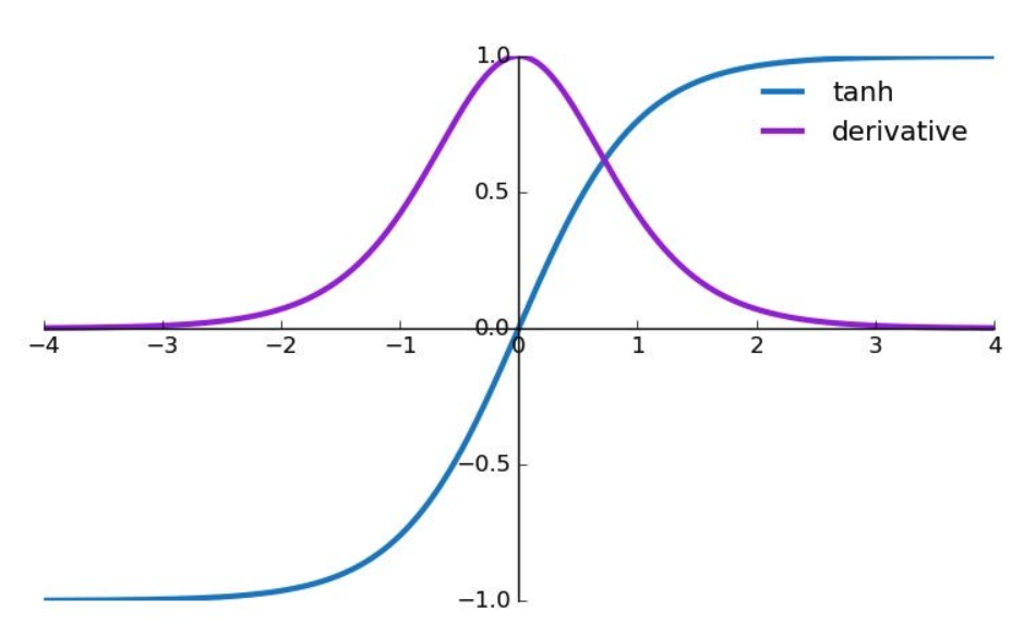
  • The vanishing gradient problem often arises when using certain activation functions like the sigmoid function or hyperbolic tangent (tanh) function

    

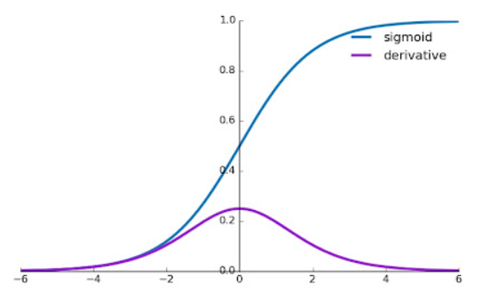
  • For large positive or negative inputs to the sigmoid function, the sigmoid function “saturates” near 0 or 1, where the derivative is a very small positive number
  • For large positive or negative inputs to the tanh function, the tanh function “saturates” near -1 or 1, where the derivative is a very small positive number.
  • During backpropagation, the local gradients are continually multiplied together, shrinking the values towards zero
  • Vanishing gradients are largely solved by techniques like:
    • Rectified Linear Unit (ReLU) activation function whose derivative is 1 for all positive inputs
      • $ReLU(x) = max(0, x)$
    • Normalized initialization and intermediate normalization layers
    • Residual networks (this paper)
• Degradation
  • As the depth of the network increases, accuracy saturates and then degrades rapidly
  • Unexpectedly, this is not caused by overfitting, and adding more layers leads to higher training error

Residual Networks

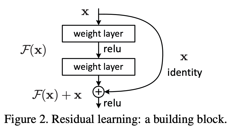
• Instead of hoping a few stacked layers directly fit a desired underlying mapping, we let these layers fit a residual mapping
  • Formally, let the underlying desired mapping be $\mathcal{H}(x)$
  • Then the stacked nonlinear layers fit a mapping of $\mathcal{F}(x) \coloneqq \mathcal{H}(x) - x$
  • The original mapping is now recast into $\mathcal{F}(x) + x$
• The hypothesis is that it is easier to optimize the residual mapping than to optimize the original, unreferenced mapping
• To the extreme, if an identity mapping were optimal, it would be easier to push the residual to zero than to fit an identity mapping by a stack of nonlinear layers
• For the implementation, we use shortcut connections which simply perform an identity mapping, and their outputs are added to the outputs of the stacked layers
• Identity shortcut connections add neither extra parameter nor computation complexity